Visibility-driven Polygon Rendering for Interactive Virtual Colonoscopy

Michael Knapp

knapp@cg.tuwien.ac.at

Institute of Computer Graphics and Algorithms
Vienna University of Technology
Vienna / Austria

Abstract

This paper describes an implementation of a surface based rendering algorithm used for virtual colonoscopy. The colon surface data is acquired by extracting a surface from computer tomography data sets. The connectivity meshes of the resulting triangles are reconstructed to determine which parts of the iso-surface belong to the colon. Further the colon is intersected into a number of pieces along its center-line. Then these pieces are rendered depending on their visibility using graphics hardware capable of triangle rasterisation. The implementation of the rendering algorithm is embedded into the virtual endoscopy environment VirEn.

Keywords: virtual endoscopy, colonoscopy, surface based rendering.

1. Introduction

With 160 cases per 100,000 inhabitants colon cancer is the second leading cause of cancer deaths in Europe. One effective diagnostic method to detect malignant polyps or tumors is optical endoscopy. After cleaning the colon and inflating it with air a fiber optical probe with a tiny camera and light source attached to its tip is introduced into the colon. Then, physicians examine the inner surface of the colon by manipulating the position of the camera on the probe tip. This invasive procedure takes about one hour and is expensive and quite discomfortable for the patient.

Virtual Colonoscopy is an alternative non-invasive method to optical colonoscopy, with less expense, reduced patient discomfort and potentially improved diagnostic sensitivity. First, the patient’s colon is cleaned and inflated with air. Second, a computer tomography scan of the abdomen is taken which generates a three-dimensional data set covering the entire range of the colon. Third, the colon surface is extracted from the data set. The physician can virtually examine the colon surface by navigating a virtual camera.

This paper describes a surface based approach for interactive (at least 10 frames per second) virtual endoscopy. Today, common low cost graphics hardware supports efficient rendering of thousands of triangles per second. The surface of the colon, consisting of millions of triangles, is too large to deal with to achieve interactive frame rates. Actually we have to render only those triangles, which are visible from the current view position. Because of the tube like structure of the colon, the number of the visible triangles is far less than the total number of triangles.

The reduction of triangles by merging adjacent triangles leads to information loss, e.g. small polyps will disappear, which is an unwanted effect of this method. So we cannot use any algorithms, which can cause the loss of important details.

First a computer tomography scan of the body part, which will be examined later, is generated. Then an iso-surface extraction algorithm [6] is applied to extract the colon triangle data. In practical cases the colon data consists of several millions of triangles. After extracting the iso-surface with the existing marching cubes implementation in VirEn [9], which outputs a list of disconnected triangles, the connectivity of the triangles has to be reconstructed to determine the colon surface.

This paper describes the implementation of many ideas of the rendering method proposed by Hong et al. [2]. Contrary to [2], our paper puts the emphasis on the preprocessing step instead on the rendering step.

2. Related Work

In the field of virtual endoscopy, various approaches to interactive virtual endoscopy exist: Hardware assisted volume rendering approaches are described in [3, 4, 5, 10] using the VolumePro rendering hardware. The VolumePro hardware used for the implementation does not support perspective projection, so perspective volume rendering is approximated by an algorithm which combines multiple base plane images, parallel projections of the slabs, generated by VolumePro board, with perspective projected texture rendering.

An image-based approach, where the current visible section of the colon is mapped onto a cube, which can be unfolded, is described in [8]. From the six possible directions in a cube volume rendered images are generated and used as a cubic environment map. The current view position is in the center of the cube. By unfolding the cube it is possible to view the complete surroundings of the current view position, which improves the examination efficiency.

Direct volume rendering is combined with surface based rendering techniques in [11, 12]. The colon surface is rendered by ray-casting the data in the neighborhood of the colon surface. This surface assisted technique helps to skip most of the empty space within a colon to reduce the calculation time.

Surface rendering with a special volume ray-casting hardware called VIZARD II is described in [7]. The colon surface can be rendered opaquely or translucently with this hardware and it is possible to achieve interactive frame rates.

3. The Preprocessing Step

The surface extraction algorithm marching cubes generates millions of triangles from volume data sets used in virtual endoscopy. This large number of triangles cannot be displayed at an interactive frame rate, so a way has to be found to display only the visible triangles depending on the current view position and direction.

In this section we describe an algorithm for reconstructing meshes from a list of disconnected and unsorted triangles. A mesh that consists of a set of connected triangles we call a component. A component is represented by a structure containing a list of vertices, a list of normals (one normal per vertex) and a list of triangles. Each triangle contains three indices into the vertex list respectively the list of vertex normals.

This section describes following algorithm: First, the iso-surface is extracted, in the second step a plane along the center-line intersects the set of triangles. This plane divides the whole triangle set into two parts. On the part that is on the ‘side of interest’ the mesh reconstruction step is applied to figure out the components. The other part is ignored. For the component, which contains a portal line, the mean point of the vertices of the portal line is calculated. The mean points of the components are compared with the current position on the center-line. The component with the mean point, which has the shortest distance to the current position on the center-line will be the new cell.

3.1 Surface Extraction

A widely used iso-surface extraction algorithm is the marching cubes algorithm [6]. It is also used in VirEn [9]. The marching cubes implementation of VirEn outputs a list of unsorted and disconnected triangles (Figure 1, on the left). Each triangle contains three vertices and for each vertex a normal is stored.

The result is a list of triangles, but their connectivity is unknown. For deciding which parts belong to the colon, we have to know the connectivity of them. Parts, which do not belong to the colon, will never be seen, so we can remove them to reduce the overall number of triangles. One good way to find out the connectivity is to reconstruct triangle meshes from these triangles.

3.2 Topology – Mesh Reconstruction

In the following sections we describe the steps needed for reconstructing the triangle meshes from a list of disconnected triangles. The result of these steps is a list of components. Each component contains a connected triangle mesh (see Figure 1, on the right).

3.2.1 Preparing the mesh reconstruction

First, we create two arrays from a list of N triangles: one array, the vertex array, containing the vertices of these triangles, that are N*3 vertices, and another array, the triangle array, containing N triangles. Each vertex in the vertex array points to its triangle in the triangle array, and each triangle points to its three vertices in the vertex array.

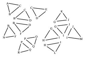
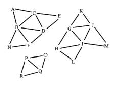
Figure 1: Input triangles and the expected output, the components, represented by connected triangle meshes

We assume that vertices with the same coordinates represent a single vertex in a mesh. That means, that all triangles, which have this vertex as a coordinate, belong to this mesh. To find out these vertices, which have the same coordinates, the vertices of the triangles are put together into groups. A group is a block of vertices with the same coordinates in the vertex array. One fast way to achieve that is to sort the vertices. A fast sorting algorithm is quicksort [1]. The effect of sorting is, that vertices with the same coordinates are clustered together into a block. The sorting criteria must be chosen that way, that all vertices with the same coordinates are clustered into a single block. One criterion can be the distance between the coordinates, another is the sorting according to the x coordinate, then sorting within same x coordinates according to the y coordinate, and within same y coordinates according to the z coordinate. The last mentioned criterion is used in the implementation we describe here. After grouping the vertices by sorting the vertex array, we number the groups starting from zero by setting the group field of each vertex in the vertex array. These steps are illustrated in Figure 2.

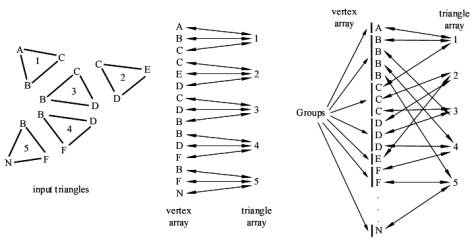
Figure 2: The input triangles on the left and the resulting vertex array and triangle array with their references to each other are shown before the vertex array is sorted. The vertex array is shown on the right side after sorting. The vertices are clustered into the so-called groups.

3.2.2 Creating the Components

We expect that our triangle data set consist of several disconnected meshes. To find out these meshes, represented by the so-called components, one vertex from the vertex array is taken, then its group, which the vertex belongs to, is determined. For each vertex of the group, if the vertex is not "visited" (each vertex in the vertex array has a "visited" flag), we look at the triangle, which this vertex belongs to. If this triangle is not "visited" (each triangle in the triangle array has a "visited" flag, too), we mark this triangle as "visited", and push its vertices onto the stack. Below, Algorithm 3.1 describes this step with a pseudo code program.

( 0) // Algorithm for creating components

( 1) component = 0

( 2) for (all vertices) do

( 3) {

( 5) if (vertex.visited == false) then

( 5) {

( 6) stack.push(vertex)

( 7) while (stack.empty == false) do

( 8) {

( 9) vertex = stack.pop()

(10) if (vertex.visited == false) then

(11) {

(12) group = vertex.group

(13) for (each vertex in group) do

(14) {

(15) vertex.component = component;

(16) vertex.visited = true

(17) }

(18) for (each vertex in group) do

(19) {

(20) triangle = vertex.triangle

(21) if (triangle.visited == false) do

(22) {

(23) triangle.visited = true

(24) triangle.component = component

(25) stack.push(triangle.vertex1)

(26) stack.push(triangle.vertex2)

(27) stack.push(triangle.vertex3)

(28) }

(29) }

(30) }

(31) }

(32) component = component + 1

(33) }

(34) }

Algorithm 1: Algorithm for creating the components. Input are the sorted vertex array and the triangle array as described in 3.2.1. The algorithm modifies the ‘component’ fields of the vertices and the triangles in both arrays.

3.3 Cell Generation

In this section we describe how the cells are created. Algorithm 2 depicts the pseudo code describing the following steps.

3.3.1 Intersecting the Colon

As mentioned above, displaying all triangles at an interactive frame rate is not possible.
Because of the tube like structure of the colon, only a small section of the whole colon is visible. If the colon is parameterized from 0 to 1, thus the potentially visible section (Figure 3: ‘potentially visible section’) ranges from t₁ to t₂, with 0 £ t₁ < t₂ £ 1 is potentially visible.

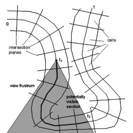
Figure 3: Potentially visible section of the colon

The idea is to cut the colon into N pieces, the so-called cells. The continuous parameter space can be mapped into the discrete cell ‘space’, which ranges from 0 to N-1 by a function

f(t) = { i | cell[i].start £ t < cell[i].end : 0 £ i £ N-1 }.

To display the visible section of the colon only cells from f(t₁) to f(t₂) need to be displayed.

3.3.2 Creating the Cells

The colon is intersected along the center-line, which is supplied by VirEn, by fixed length steps. We intersect the colon along this center-line by a plane (Figure 4: ‘Intersection Plane’), whose normal equals the tangent of the center line at its intersection point with the plane. The position of the plane is determined by the current position on the center-line (Figure 4: ‘Position on Center Line’, dot on ‘Intersection Plane’ and center line). All vertices and the triangles on the opposite side of the intersection plane are marked as “unused” (Figure 4: white area below the ‘Intersection Plane‘). Triangles belonging to cells, which were created previously (Figure 4: ‘Existing Cells’, dark gray area) are ignored and not used any more for further cells. On the triangles that will contain the new cell the mesh generation algorithm is applied as described in chapter 3.2. The result is a number of components (Figure 4: ‘Current Components’, light gray area)

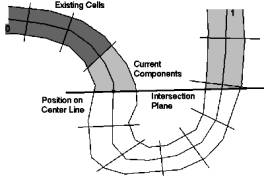
Figure 4: Intersection plane

After this step a number of components have been created, but only one of them will become the new cell. The component, which becomes the new cell, has to be figured out.

Each cell has two portals. A portal is represented by a series of vertices, which usually make up a line (Figure 5: thick zig-zag line), which consist of the border edges of the border triangles of the component. Only Triangles, which have only two vertices (Figure 2: triangles with the number 2) on the "side of interest" of the intersection plane (Figure 5: straight thick line) have a border edge. The vertices of the border-line will be used for calculating the culling rectangle, which is used for rendering. The culling rectangle is explained in section 4.

In our algorithm we calculate the mean point of all vertices of this line. This mean point is very close to the intersection point of the plane and the center-line, which is the current position on the center-line (Figure 4: ‘Position on Center Line’, dot on ‘Intersection Plane’ and center-line). The mean point of the portal line of the new cell has the smallest distance from the position on the center-line from all components (Figure 4: light gray area).

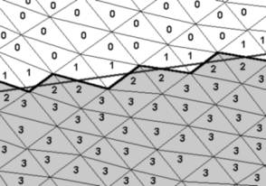
Figure 5: This figure shows, how the triangles are classified in the intersection step. The numbers denote the number of vertices on the “side of interest” (gray triangles). Triangles with one and no vertices are marked as “unused”. The border-line (black thick zig-zag line), intersection plane (straight thick gray line) are also shown.

Finally we have figured out our new cell. From each cell we point to its “back portal” and “front portal. In this step only one new portal, the “front portal” has been created, but a cell has two portals. The “back portal” of the new cell is the “front portal” of the previously created cell.

After this step we mark all vertices in the vertex array, which belong to this new cell. We do so by setting the “cell” flag of the vertices.

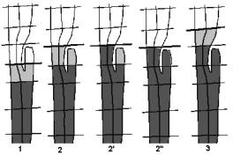
Figure 6: special case handling

3.3.3 Special Cases

For this algorithm, handling of special cases is also necessary. The main problem is some unusual structures of the colon, or cut-off artifacts appearing during the intersection. Figure 6 shows such a special case, whose handling is described step by step.

1. The cells are created as described in 3.3.2 . The component is recognized to be the new cell, but it is unknown whether its portal consists of more than one closed border-lines. Usually a portal is represented by a single closed border-line, so every additional border-line is an unwanted hole. The vertices of extra border-lines are added to the set of vertices of the existing border-line of the portal of the cell to be created.

2. The next intersection is applied. The components are created again as described above. (Algorithm 2: Steps (5) to (9))

2'. The cell is created. (Algorithm 2: Steps (10) to (15))

2". A check is applied on the other components, whether they contain any vertices that belong to an existing cell. We check every vertex of the component, whether the “cell” flag is set or not. When marked vertices are found, the component is added to the new cell, otherwise the component is ignored. (Algorithm 2: Steps (16) to (24))

3. Cell creation continues with the next intersection.

3.3.4 Postprocessing

After a cell has been created, triangle strips are generated from its triangles. Rendering triangle strips is supported by nearly all consumer graphics hardware and shows a much higher performance than rendering single triangles.

Below, in Algorithm 2 all cell creation steps are described in pseudo code.

( 0) // Algorithm for creating the cells
( 1) back_portal = null

( 2) parameter = center_line.begin

( 3) while (parameter < center_line.end) do

( 4) {

( 5) position = center_line.position_at(parameter)

( 6) plane.normal = center_line.direction_at(parameter)

( 7) plane.point = position

( 8) intersect_triangles(plane, vertices, triangles,

important_vertices, important_triangles)

( 9) create_components(important_vertices, important_triangles)

(10) component = find_component_at_position(important_vertices,

important_triangles, position)

(11) cell = create_cell_from_component(component)

(12)    front_portal = create_portal_from_component(component)
(13)    front_portal.position = position
(14)    mark_as_cell_vertices(vertices, component)

(15) remove_component_from_triangles(component, vertices, triangles)

(16) for (all components) do

(17) {

(18) if (component_contains_cell_vertices(component)) then

(19) {

(20) mark_as_cell_vertices(vertices, component)

(21) add_component_to_cell(component, cell)

(22) remove_component_from_triangles(component,

vertices, triangles)

(23) }

(24)    }
(25)    cell.back_portal = back_portal
(26)    cell.front_portal = front_portal

(27) cell_list.insert_cell(cell)
(28) back_portal = front_portal;

(29) parameter = parameter + step_forward

(30) }

Algorithm 2: This algorithm describes the partitioning of the colon into cells. The input is the sorted vertex array, the triangle array and the center-line. The output is a list of cells.

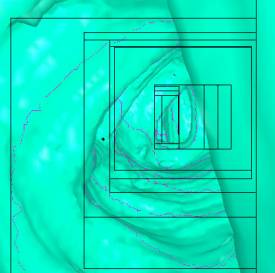
4. The Rendering Step

First, we determine the cell, which contains the current camera position. This cell is determined by checking the current camera position with the position of the back portal and the front portal.

At the beginning this cell is drawn and the culling rectangle is set to the displayed area size. Then the bounding rectangle of the portal between this and the next cell is calculated and is intersected with the culling rectangle. The resulting rectangle becomes the new culling rectangle. Further the culling rectangle is reduced by checking the Z-buffer [2].

One advantage of the portal based rendering is, that as long the viewing position stays inside the colon, the algorithm works as expected. The navigation is not restricted to view positions on the center-line. Thus it is possible to move freely within the colon.

5. Results

The algorithm was implemented using Microsoft Visual C++, and tested on an AMD Athlon 600Mhz system, 512 megabytes of RAM, and an nVidia Geforce256 graphics adapter.
The Gouraud shaded triangles are drawn using the OpenGL graphics library as triangle strips.

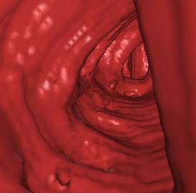
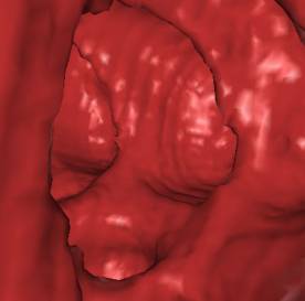
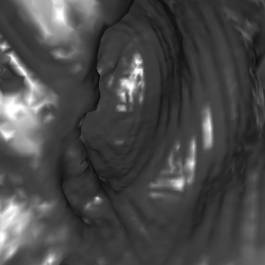
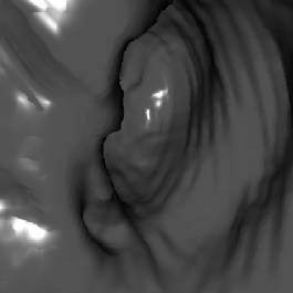
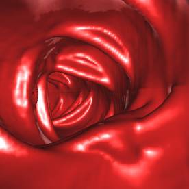
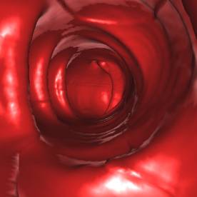
Table 1 shows some numbers evaluated during the test of the implementation. The following figures (Figure 7 - 10) show some sample views of the colon data sets used for testing.

Size of data set	Total Number of triangles	Total Number of triangles in cells	Number of cells	Total Number of triangle strips	Average number of triangles per strip	Preprocessing time [s]	Minimum frame rate [s^-1]
198x115x300	69.824	36.083	50	1239	29	9	38
198x115x300	161.346	82.844	50	2152	38	24	27
198x115x300*	652.704	333.158	50	6539	50	148	10
198x115x100	377.636	109.683	16	2569	45	88	11
381x120x632	894.478	632.075	76	11838	53	356	15
381x120x632	945.132	690.863	77	12523	55	421	14

Table 1: Preprocessing and rendering statistics
*) Figure 7, 8, and 9 show sections of this data set

6. Conclusion

It was possible to achieve interactive frame rates while maintaining a reasonably visual quality using this surface rendering technique. With better hardware (currently nVidia Geforce 4 and 2GHz CPUs) it will be possible to render the colon surface with a higher triangle count, which improves the quality, so that it will reach the quality of ray-casted images.

Rendering only the visible cells is a great improvement over brute-force rendering. Further, the number of cells to be drawn can be reduced by minimizing the size of the portals of the cell. One way is searching for constrictions in the colon, the transitions between two bulges of the colon, the so-called haustra.

Using a marching cubes implementation that retains the connectivity of the iso-surfaces can speed up the preprocessing step. Another improvement would be the removal of structures that will be never visible because they do not belong to the colon surface. This removal step shall take place before the cell generation step starts. The removal procedure reduces the number of triangles to be processed, thus the preprocessing time.

This portal based rendering method can be easily extended for branched structures, so this algorithm can be used for bronchoscopy and other types of endoscopy where branched structures occur.